The gamer's guide to line algorithms
If you’ve ever tried making your own roguelike, you’ve likely encountered all sorts of strange-looking 1960s algorithms for doing geometry. Bresenham’s line algorithm is the most famous, but you often see people talking about “DDA lines” among other things. Hopefully, you found your way to the excellent Red Blob Games article on the subject, which describes a modern implementation in detail, with lovely interactive examples.
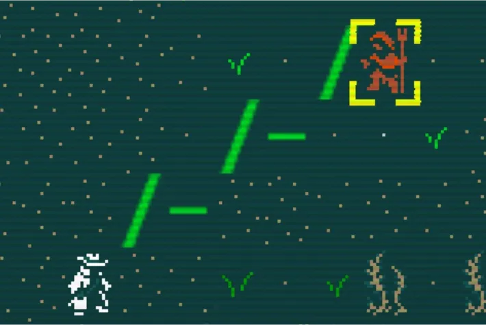 A line algorithm used to menace an innocent watervine farmer
Perhaps this left you with unanswered questions. These vintage functions look so different from each other, but they all seem to do the same thing!
This post is structured as an ahistorical journey back through time. We start with the floating point algorithm given by Red Blob, which is optimal on modern computers, and end at Bresenham’s 1962 algorithm which uses pure integer arithmetic, as was optimal on the hardware of the day. We can then consider the other functions as steps along our imagined refactoring process, replacing floats piece by piece with integers.
The aim is to present these functions in a unified style so they can be easily compared, and to try and give a little intuition as to what is going on with the geometry.
Linear Interpolation Line
function lerpLine(start, end) {
  let points = [];
  let length = diagonal_distance(start, end);

  for (let i = 0; i <= length; i++) {
    let t = i / length;
    points.push(round_point(lerp_point(start, end, t)));
  }

  return points;
}
This is the Linear Interpolation or lerp line, as given in the Red Blob article. If you’re not familiar with lerp() and what it does, you should take a look through that article. It goes through it in detail and was a big inspiration for this post.
Let’s write it out longhand in rust, so we can see the types:
struct Point {
  x: i32,
  y: i32,
}

fn lerp_line(start: Point, end: Point) -> Vec<Point> {
  let delta_x = end.x - start.x;
  let delta_y = end.y - start.y;
  let length = delta_x.abs().max(delta_y.abs());

  (0..=length).map(|step| {
    let t = step as f32 / length as f32;
    let x = t * delta_x as f32 + start.x as f32;
    let y = t * delta_y as f32 + start.y as f32;

    Point::new(x.round() as i32, y.round() as i32)
  })
  .collect()
}
NOTE: In all these examples, anything that doesn’t have f32 next to it is an integer, its type having been inferred from the Point definition.

The blue squares in my wonderful diagram are the final set of tiles, called the “digital line”. The red line is the real line. It’s both the “real” line in the sense that it’s a proper, sensible straight line between two points, but also because it’s defined using $\mathbb R$eal numbers, i.e. decimals that we represent using floating point.
This is the “ideal” line from $start$ to $end$, and in all these functions our task is to find the digital line (set of tiles) that follows it most closely.
The setup
Let’s look at the initialization part of the function first:
let delta_x = end.x - start.x;
let delta_y = end.y - start.y;
let length = delta_x.abs().max(delta_y.abs());
delta_x and delta_y, aka $\Delta x$ and $\Delta y$, are the “width” and “height” of the line, shown on the left by the black dotted lines. (Delta means difference, or change.) This is how far we need to go in each direction to get from $Start$ to $End.$
length is the total length of the line, which we take to be the longest of $\Delta x$ or $\Delta y$, which seems weird! Shouldn’t we be using $\sqrt{\Delta x^2 + \Delta y^2}$ to find the hypotenuse, per Pythagoras? No, because here we’re measuring the digital line, not the real line. Roguelike developers are familiar with the need for different distance metrics when working on the grid, and might recognize this calculation as the Chebyshev distance.
This is the metric that describes the geometry of an 8-connected grid, where a diagonal move is the same distance as a cardinal move. We use Chebyshev distance here because it corresponds to the number of discrete steps needed to move from one tile to another when diagonal moves are allowed, making it perfect for line rasterization. This differs from the real world where the diagonal across a square is longer than the sides.
The lerp
(0..=length).map(|step| {
  let t = step as f32 / length as f32;
  let x = t * delta_x as f32 + start.x as f32;
  let y = t * delta_y as f32 + start.y as f32;

  Point::new(x.round() as i32, y.round() as i32)
})
This is where the actual interpolation happens. step is proceeding from $0$ to $length$, and so by dividing $\frac {step} {length}$ we know how far through the line we are. We call this $t$ for time, even though here we’re not actually thinking about movement.
In the diagram I’ve added the green crosshairs to show the calculation for the 6th tile, when step == 5. As $t$ is a decimal between zero and one we can just multiply that by $\Delta x$ to get our $x$ coordinate, and respectively for $y$. Finally, we add the start coordinate back in to offset the line to the correct position.
The round
So, we’ve interpolated our $(x,y)$ points, shown by the red dots. We can see that these are perfectly on the real line. Now we just need to round() them to get the tiles in the digital line. This is depicted by the blue dots joined to the red dots by the little blue lines. Sometimes they get rounded by more, sometimes less, and sometimes they’re bang on and the rounding does nothing.
Looks good to me?
There’s the division to compute t right there in the loop. A bit of refactoring could move that up into the setup phase. In real life that kind of thing is the compiler’s problem, and you should write your code however is clearest and simplest. For the sake of our exploration, let’s see what it would look like.
Vector Line
fn vector_line(start: Point, end: Point) -> Vec<Point> {
    let delta_x = end.x - start.x;
    let delta_y = end.y - start.y;
    let length = delta_x.abs().max(delta_y.abs());

    let unit_displacement_x = delta_x as f32 / length as f32;
    let unit_displacement_y = delta_y as f32 / length as f32;

    (0..=length).map(|step| {
        let x = step as f32 * unit_displacement_x + start.x as f32;
        let y = step as f32 * unit_displacement_y + start.y as f32;

        Point::new(x.round() as i32, y.round() as i32)
    })
    .collect()
}
lerp() can return correct values for any t which is why it’s so useful, but we’re working with fixed intervals along the line, always exactly one tile apart. This means we can precalculate a single increment for each axis before we start and then multiply it by step on each iteration.
In geometry terms, we’ve defined the line as a vector comprised of $\Delta x$ and $\Delta y$. This is called a displacement vector, and it represents the line’s direction and length separate to its position in space. We divide the displacement vector by the total length of the line, to get a unit vector. This is called “normalizing” it.
Note that once again we’re calculating the length of the line using the Chebyshev distance metric, because we’re working on the grid. Typically, you would normalize a vector using the Pythagoras-style length formula, called the $L_2$ or Euclidean norm, yielding a vector with Euclidean length 1. Here we’re using the $L_\infty$ or Chebyshev norm, which gives us a vector with Chebyshev length 1. This is suited for our grid-based line drawing, where we want to measure distance in terms of grid steps.
From then on we proceed much the same way as with the lerp line, except it’s simpler as we have this single precalculated interval representing the displacement of the real line between each tile. We just need to multiply that by the step counter, add the start point back in again to offset the line in world-space, and then round() as before.
In reference to the diagram, the unit displacement vector represents the distance between two of the red dots. The regularity of those dots cannot by now have escaped you. They’re not just evenly spaced: they’re precisely on the grid lines, at least along the $x$ axis, which brings us to the…
Digital Differential Analyzer Line
pub fn dda_line(start: Point, end: Point) -> Vec<Point> {
    let octant = Octant::from_points(start, end);
    let start = octant.to_octant0(start);
    let end = octant.to_octant0(end);

    let delta_x = end.x - start.x;
    let delta_y = end.y - start.y;
    let slope = delta_y as f32 / delta_x as f32;

    (0..=delta_x).map(|step| {
        let x = step + start.x;
        let y = step as f32 * slope + start.y as f32;

        octant.from_octant0(Point::new(x, y.round() as i32))
    })
    .collect()
}
With the DDA line we’re getting to the historical algorithms, and the quest to replace floating point with integer math begins.
Astute viewers may have noticed that when calculating our vector, we divided both delta_x and delta_y by length, but we defined length as being equal to either delta_x or delta_y. This means one of them is always going to be divided by itself and so equal to 1. In the loop we’re then multiplying by 1, effectively a no-op. This redundancy is our next target for “optimization”. We’re going to turn these invariants into assumptions.
With the DDA line, we assume that the longest dimension is always going to be along the $x$ axis, and so length == delta_x. Thus, when we normalize it we’re dividing it by itself, giving an increment of exactly 1. Thus, incrementing x just means adding 1 at every step, removing another floating point calculation.
For the y axis, we multiply step (which is now just the x coordinate) by the slope, which is simply the value that would previously have been in the $y$ component of the displacement vector. We have arrived at the classic $y = mx + c$ slope-intercept line formula from school, where $m$ is the slope and $c$ is start.y.
Octants?
All the octant stuff is how we get away with assuming that $x$ is always the longest dimension. We just mirror/flip the points around until that’s the case, and then flip them back again at the end, using a bunch of if statements. There are other ways of solving this problem that you see around, and they amount to inlining those same conditionals into the body of the function. You often see a sign variable that’s set to either -1 or 1 and used to orient the line.
Helpfully this means that we don’t need to call abs() any more, as the lengths will always be positive.
If you set this up carefully to keep all the conditionals out of the loop, it can be faster. If you do it carefully to the DDA algorithm, you obtain the so-called Extremely Fast Line Algorithm, variant B. I’ve used the octant transform in all these examples as it does the least damage to the algorithm’s structure.
The code for the octant functions is available here.
 Only girls were allowed to use computers back in the day
What exactly is a “Digital Differential Analyzer” anyway?
A differential analyzer is a mechanical calculator from the black and white times. It’s basically a giant gearbox that uses gear ratios to solve differential equations.
A digital differential analyzer is a solid-state implementation of the same thing. It was the last iteration of these antique machines before the modern stored-program computer. Have a look at the wiki article, and you’ll see the resemblance to our line functions.
Fractional Accumulation Line
pub fn fractional_accumulation_line(start: Point, end: Point) -> Vec<Point> {
    let octant = Octant::from_points(start, end);
    let start = octant.to_octant0(start);
    let end = octant.to_octant0(end);

    let delta_x = end.x - start.x;
    let delta_y = end.y - start.y;
    let slope = delta_y as f32 / delta_x as f32;

    let mut y = 0;
    let mut accumulator = 0.0;

    (0..=delta_x).map(|step| {
        let point = Point::new(step + start.x, y + start.y);

        accumulator += slope;

        if accumulator >= 0.5 {
            y += 1;
            accumulator -= 1.0;
        }

        octant.from_octant0(point)
    })
    .collect()
}
This one I’m featuring merely as a step in our derivation, I don’t think it was used in practice.
As you can see, both the x and y variables are now integers, there are no calls to round() remaining, and instead we have this one floating point accumulator variable. We use that to “save up” the fractional y coordinate increments across iterations of the loop, and when we’ve got enough for another tile we “spend” it by incrementing y by a whole unit and then subtracting from our “balance” in the accumulator.
Note that we take 0.5 as the threshold for the next tile because that’s when we’re halfway through the tile and it’s time to snap to the next one, exactly how rounding works. We’ve basically written out the rounding operation by hand. If you’ve heard of the “midpoint line algorithm”, then that $0.5$ halfway point through the tile is the “midpoint” being referred to in the name. That brings us neatly on to…
Bresenham’s Line
pub fn bresenham_line(start: Point, end: Point) -> Vec<Point>
    let octant = Octant::from_points(start, end);
    let start = octant.to_octant0(start);
    let end = octant.to_octant0(end);

    let delta_x = end.x - start.x;
    let delta_y = end.y - start.y;
    let mut error = 2 * delta_y - delta_x;
    let mut y = 0;

    (0..=delta_x).map(|step| {
        let point = Point::new(step + start.x, y + start.y);

        if error > 0 {
            y += 1;
            error -= 2 * delta_x;
        }

        error += 2 * delta_y;

        octant.from_octant0(point)
    })
    .collect()
}
 Jack B himself.
Now that all the floating point representations have been squeezed down into this single variable, we’re well placed to get rid of it completely.
There are two things necessitating the remaining floating point math that we need to get rid of. First is the comparison with 0.5. We avoid this by simply multiplying all the relevant values by $2$, so we can compare with 1 instead.
We actually end up using 0 rather than 1 - it works out the same and using 0 is considered more “natural”. Initializing the y_accumulator to -delta_x is what makes this work. If you try and start the accumulator at zero and compare with 1, you still get a straight line, but it looks weird and doesn’t match the other algorithms’ output.
The second issue is the slope variable. We can see that it was previously defined as $\frac {\Delta y}{\Delta x}$, but this division is the last remaining floating point operation, so it has to go. We do a quick bit of algebra and cancel it out by multiplying all the relevant values by $\Delta x$, basically the same trick again. With that, we’ve reached a pure integer math implementation!
What is going on here?
As we’ve seen, there are multiple ways to describe a line (or any shape) mathematically, and we can use each of them in different ways to draw the same thing, depending on what we’re trying to do.
Implicit form
\[ax + by + c = 0\]In this definition, the line is all the points for which this equality holds true. $a$ and $b$ describe the slope in each dimension (related to our $\Delta x$ and $\Delta y$ values) and $c$ is the offset from the origin.
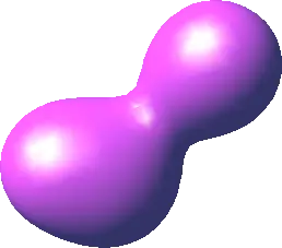 The classic 1990s "metaball" goo shapes are drawn using an implicit equation
This is similar to how things are set up in our Vector Line algorithm. However, it’s a bit weird - it only tells us how to check if a given point is on the line or not. We can’t actually use this formula to iterate over the points on the line like we want to. You’d have to iterate over every single point inside the bounds, check if the equality holds, and pick those tiles. That would be very inefficient!
Imagine instead that you’re not drawing a line, but some wobbly shape. Perhaps you’ve generated it using some weird technique, and you don’t even know in advance what it looks like. In that case, an implicit formula is just what you need, as you’ll need to check every point anyway.
Also good if you’re writing a GPU shader, which runs for every single pixel at the same time.
Explicit form
\[y = mx + c\]This is the aforementioned formula you may or may not remember from school. $m$ is the slope (this time as a single number) and $c$ is still the y-offset. This is much more appropriate to our purposes, because it actually tells us directly what one of the coordinates is going to be, in this case $y$. It does rely on us already knowing the other coordinate, but as we’ve seen with the DDA line, that’s actually possible in many situations.
Parametric form
\[x = x_0 + ta\] \[y = y_0 + tb\]This is the form we started with in the Linear Interpolation and Vector Line algorithms. The parametric form describes the line using a single parameter $t$ (the “time”) which represents how far along the line we are. When $t = 0$, we’re at the ${start}$, and when $t = 1$, we’re at the ${end}$. The values $a$ and $b$ correspond to our $\Delta x$ and $\Delta y$ respectively.
What makes this form particularly useful for line drawing is that we can easily generate points at regular intervals by stepping $t$ from $0$ to $1$. This is exactly what we did in the lerp algorithm, where we calculated $t = \frac{step}{length}$ and then plugged it into these equations.
The parametric form is also especially convenient when you want to extend the line beyond its endpoints, as you’re free to set $t > 1$ or $t < 0$.
The punchline
If you hated the endless calculations they tried to make you do in school and learned most of your maths on the computer, you might think of lerp() as just a handy way of finding intermediate values between two extremes. You’ve used it to draw color gradients, fade sounds up and down, have monsters follow the player and basically everything else.
You’re broadly aware that the “Linear” part in the name refers to the fact that lerp() has the output change at a constant rate, without accelerating or decelerating on the way from 0 to 1. If you want that behaviour, you know to modify the t parameter with an “easing function”, which typically squares it or cubes it. Presumably this is what makes it not linear any more, which makes sense, despite the fact that you’re still calling a function called lerp().
On top of that, you know from music software that simple DSP processes are “linear”, in that the absolute input level doesn’t affect the nature of the processing. You know that “nonlinear” processors, where you have to watch the input gain, are somehow fundamentally more exotic and require CPU-intensive oversampling.
It turns out that what the “linear” in “linear interpolation” really says is that this simply is the function describing a line in Euclidean space. It’s not some approximation, or some kind of clever technique: what you get when you linearly interpolate from point A to point B is an honest-to-goodness line, direct from the platonic realm to your computer. The map is the territory after all!
Other weird stuff you might see
Here I’ll discuss some other, even more confusing ways of writing some of this stuff that you might have seen in the wild.
Optimised Bresenham
void plotLine(int x0, int y0, int x1, int y1)
{
   int dx =  abs(x1-x0), sx = x0 < x1 ? 1 : -1;
   int dy = -abs(y1-y0), sy = y0 < y1 ? 1 : -1;
   int err = dx+dy, e2; /* error value e_xy */

   for(;;){  /* loop */
      setPixel(x0,y0);
      if (x0==x1 && y0==y1) break;
      e2 = 2*err;
      if (e2 >= dy) { err += dy; x0 += sx; } /* e_xy+e_x > 0 */
      if (e2 <= dx) { err += dx; y0 += sy; } /* e_xy+e_y < 0 */
   }
}
This beautiful Bresenham implementation comes from Alois Zingl’s page “The Beauty of Bresenham’s Algorithm”. It looks very compressed compared to our implementation, and some of that is due to the use of ternary/inline conditionals and multiple assignment to golf the logic into a smaller number of lines. Also, it’s directly calling setPixel() rather than building a list of points like we did, which makes it terser.
The most interesting thing though is the symmetry. It doesn’t assume anything about which dimension is the longest, or if the line goes left-to-right or right-to-left. Instead of using the octant transform, it has the relevant logic inlined into the function like we talked about before, in a particularly elegant way. Partly this is done with the sx and sy sign variables.
Notice that we still have just a single error value! The separation into the err and e2 variables is just an implementation detail, they both represent the same quantity. This is enabled by what Zingl calls the “xy-symmetry” of Bresenham’s algorithm. It also requires a different initial value for the error.
In their full paper, Zingl shows how this symmetry can be applied further in higher dimensions, as well as to plot different types of curves.
Path-heuristic-style Chebyshev distance
You might see the Chebyshev or diagonal distance function defined like this:
fn distance2d_chebyshev(start: Point, end: Point) -> f32 {
    let dx = (max(start.x, end.x) - min(start.x, end.x)) as f32;
    let dy = (max(start.y, end.y) - min(start.y, end.y)) as f32;
    if dx > dy {
        (dx - dy) + 1.0 * dy
    } else {
        (dy - dx) + 1.0 * dx
    }
}
or this:
D = 1
D2 = 1

function heuristic(node) =
    dx = abs(node.x - goal.x)
    dy = abs(node.y - goal.y)
    return D * (dx + dy) + (D2 - 2 * D) * min(dx, dy)
or even:
D = 15
D2 = 10

xDistance = abs(currentX-targetX)
yDistance = abs(currentY-targetY)
if xDistance > yDistance
     D2*yDistance + D*(xDistance-yDistance)
else
     D2*xDistance + D*(yDistance-xDistance)
end
None of these are relevant here. You just need max(dx, dy) for drawing lines.
These functions are taken from implementations of A* pathfinding, where tuning the distance metric is a key way by which the algorithm’s behaviour can be tweaked to taste. The D and D2 constants are setting the relative costs of orthogonal and diagonal moves. This implements the $L_p$ norm, a family of norms that includes the $L_1$ (Manhattan), $L_2$ (Euclidean), and $L_\infty$ (Chebyshev) norms we discussed earlier, with parameters to blend between them.
Next time…
In my next post we’re going to explore a totally different kind of line algorithm that’s decidedly non-geometric compared to these traditional ones. Stay tuned…